


ZEISS Microscopy

ZEISS Microscopy
Abstract
In this series "From Image to Results", explore various case studies explaining how to reach results from your demanding samples and acquired images in an efficient way. For each case study, we highlight different samples, imaging systems, and research questions.
We start the series with an analysis of vesicle trafficking in Cos7 cells.
Key Learnings:
- How to generate a high-resolution longitudinal study of vesicle trafficking within a single cell
- Explore basic observations concerning vesicle transport
- Showcase image analysis tools to segment vesicles and generate vesicle tracks to derive meaningful data to confirm our observations
Case Study Overview
|
Sample
|
Cos7 cells transiently transfected with mEmerald-Rab5a and Golgi7-tdTomato. |
|---|---|
|
Task
|
Track both types of vesicles, volume & distances over time, colocalization. |
|
Results
|
Graphic visualization of tracks and cells in a movie and resulting data as time line along track, scatter plots. |
|
System
|
ZEISS Lattice Lightsheet 7 |
|
Software
|
ZEISS arivis Pro |
Introduction


Figure A: Cellular localization of B4GALT1. Note strong accumulation in the Golgi apparatus.
Figure A: Cellular localization of B4GALT1. Note strong accumulation in the Golgi apparatus.
Figure A: Cellular localization of B4GALT1. Note strong accumulation in the Golgi apparatus.
For this case study, we selected a simple, yet analytically demanding Cos7 cell model that has been tagged with two different markers for vesicular transport: tdTomato-Golgi-7 and mEmerald-Rab5a-7.
The tdTomato-Golgi-7 fluorescent protein encodes the signal sequence of the protein Beta-1,4-Galactosyltransferase 1 (B4GALT1), which functions in the glycosylation of trans-membrane proteins and localizes mainly to the Golgi Apparatus and the cell membrane (Figure A).

Figure B: Cellular localization of RAB5A. Note the more distributed localization throughout cell compartments, and the strong accumulation in endosomes.
The mEmerald-Rab5a-7 fluorescent protein encodes parts of the Ras GTPase RAB5A. This protein is involved in vesicle trafficking and localizes mainly to endosomes and to the cytosol (Figure B).
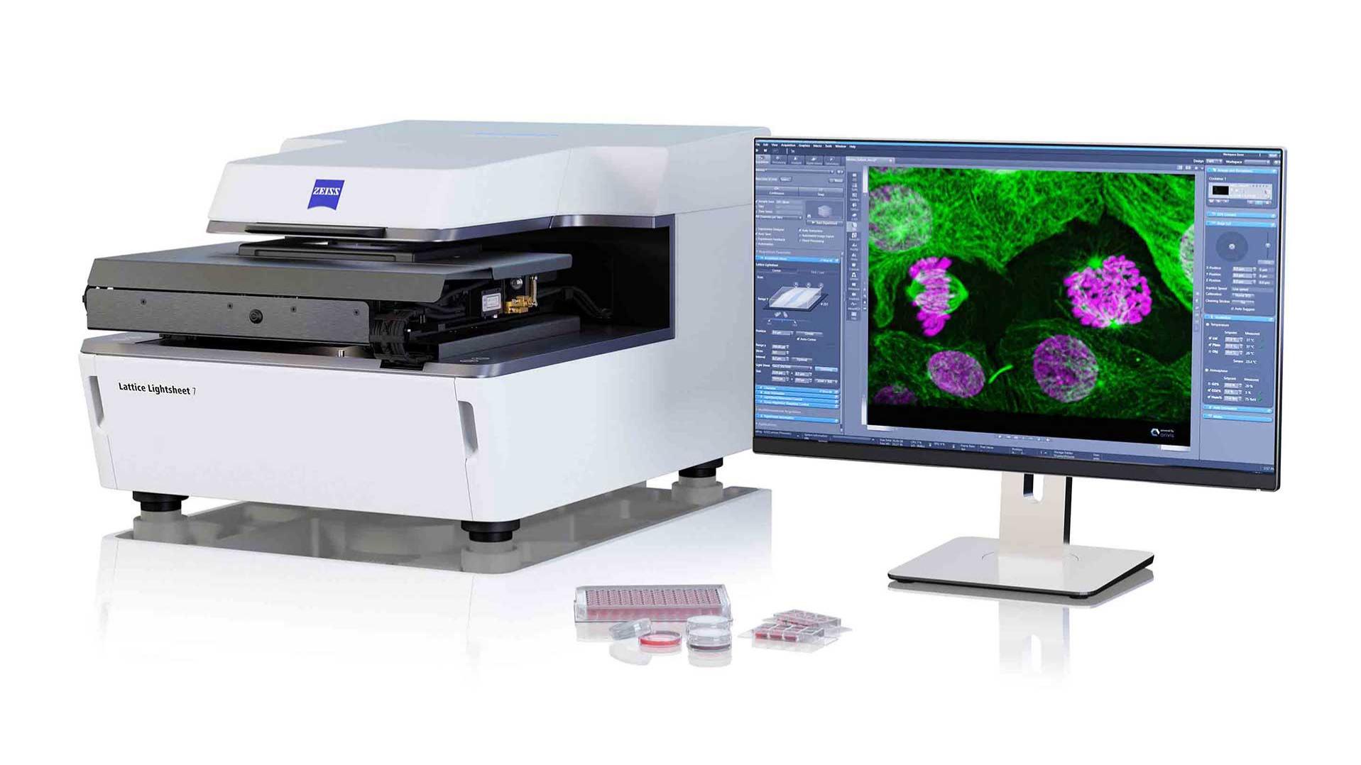

Image Acquisition
The raw data for this use case was captured with ZEISS Lattice Lightsheet 7. This system is specifically tailored for fast, volumetric live cell imaging with near-isotropic resolution, making it the perfect instrument for imaging subcellular, dynamic structures such as vesicles in 3D over time.
Using lattice light sheet microscopy, the sample is imaged at an angle, due to the geometry inherent to this technology. As a consequence, the raw data needs to be processed (deskewed) before it can be further analyzed. For this use case, 200 time points were acquired in 2 channels, one volume (85x80x20 µm³) every 3.2s, 205 planes per volume and a total of 41.000 frames in just under 11 minutes.
After acquisition, the raw data was deconvolved, deskewed and cover glass transformed using ZEN (blue edition), resulting in a processed .czi file with 0.145 µm pixel size in x, y and z. The processed .czi file could then be directly imported into ZEISS arivis Pro and converted into arivis' .sis file format, a format specifically designed for fast handling of large data sets, for further analysis.
Software Processing


Figure C: Single time-point 3D view of data set. Single channels and merge image are shown. Note the (complete) overlap of Golgi7-labelled vesicles with a fraction of the Rab5a-labelled vesicles. Also note “striping artefacts” in the green channel.
Raw Image Observation
In order to define a suitable image analysis strategy, it is important to look at the raw images (Figure C).
In this single time-point 3D representation, some imaging artifacts are visible as stripes in the green channel. As a result, some image pre-processing is necessary to remove these artifacts. ZEISS arivis Pro has two tools; “Morphology filter” and “Denoising”, which can remove these artifacts by enhancing sphere-like structures of an approximate diameter (here: ~1.5 µm) and suppressing any other signals.
Also, the images show that Golgi7-labelled vesicles strongly co-localize with a fraction of the Rab5a-labelled vesicles. In fact, careful inspection shows that there are no vesicles in the data set that are Golgi7-positive and Rab5a-negative. Hence, the dataset consists of two vesicle species: “endosomal” vesicles that are Rab5a-positive/Golgi7-negative and “Golgi-associated” vesicles that are Rab5a-positive/Golgi7-positive. The image analysis strategy needs to account for these two species by applying differential segmentation.
 overlap of Golgi7-labelled vesicles with a fraction of the Rab5a-labelled vesicles. Also note “striping artefacts” in the green channel.")
 overlap of Golgi7-labelled vesicles with a fraction of the Rab5a-labelled vesicles. Also note “striping artefacts” in the green channel.")
Figure C: Single time-point 3D view of data set. Single channels and merge image are shown. Note the (complete) overlap of Golgi7-labelled vesicles with a fraction of the Rab5a-labelled vesicles. Also note “striping artefacts” in the green channel.
 overlap of Golgi7-labelled vesicles with a fraction of the Rab5a-labelled vesicles. Also note “striping artefacts” in the green channel.")
 overlap of Golgi7-labelled vesicles with a fraction of the Rab5a-labelled vesicles. Also note “striping artefacts” in the green channel.")


Image Analysis Pipeline
In order to reduce the data size of the original raw dataset (2 channels; 150 slices; 200 time points; 16-bit; ~ 40 GB), the images were cropped to include only the relevant cellular areas. These cropped images were then used to generate a stack subset containing only every second slice and the data were then transformed to 8-bit. The final data set had 2 channels, 22 slices and 200 time points, it was 8-bit and was ~ 1.2 GB. in size.
The image analysis in ZEISS arivis Pro consisted of three steps. Firstly, image processing to denoise the images was performed, with special emphasis on preserving spherical structures and removing striping artefacts. This was done using the image processing functions “Morphology Filter” and “Denoising” independently for both channels.
Secondly, vesicles in both channels were independently segmented using Watershed segmentation with minimum vesicle volume of 0.3 µm³. The Rab5a-positive vesicles were then filtered based on the “minimal” distance to the next Golgi7-positive vesicle and assigned to the group of Rab5a-positive/Golgi7-negative “endosomal” vesicles (if distance > 0). Rab5a-positive/Golgi-positive objects were assigned to “Golgi-associated” vesicles.
Finally, to derive the movement of vesicles over time, object tracking was performed with both vesicle types.
The sketch summarizes the image analysis procedure. In addition, the ZEISS arivis Pro pipeline to perform these operations is available for download at the bottom of this page as part of the case study data package ("Green-Magenta vesicle detection_Tracking_Rev4.xml”).
Validation - Visual Track Validation
For validation of tracking, selected single vesicle tracks were examined to ensure they correctly represented the vesicle movement. In the lower panel, three tracks are shown as video sequences.Interpreting and Defining Cellular Structures
The overall distribution of vesicles helps in deducing the overall cellular architecture of the sample (Figure D). The area of high-density Golgi-associated vesicles presumably represents the main Golgi apparatus region of the cell. Next to it is a large “vesicle-free” region that represents the nuclear area. The three-dimensional contours of the nucleus can also be deduced by the spherical volume void of vesicle tracks in a 3D representation (Figure F).
A further validation is the option to visualize the cell as a “scatter plot” based on the objects’ x-y coordinates (Figure E). This shows again an accumulation of vesicles (and tracks) at the Golgi and an exclusion of vesicles from the nuclear area. This plot type is also a valuable tool for visualization of certain observations.
All other cellular regions may be assigned to “Periphery”. Assigning these areas aids a more precise description for the subsequent vesicle and track observations.


Figure D: 2D slice view on data set with vesicles
 on a scatter plot")
 on a scatter plot")
 on a scatter plot")
 on a scatter plot")
Figure E: Topological representation of vesicles and tracks (based on object x-y coordinates) on a scatter plot.


Figure F: 3D movie with visualized vesicle tracks; note the nuclear sphere in the side view.
Results
Size and Distribution of Vesicles
Having defined “endosomal” and “Golgi-associated” compartments during image analysis it is now possible to make observations and prove them with measurements and suitable visualizations.
Vesicular compartments mainly differ in size and cellular localization. The ~ 26000 identified endosomal vesicles have an average volume of 0.63 µm³, while the ~ 22000 identified Golgi-associated vesicles have an average volume of 1.062 µm³. The volume distributions are also shown in Figure G. Endosomal vesicles are devoid in the Golgi area and evenly distributed over the cell periphery (Figure H). Golgi-associated vesicles accumulate more in the central “Golgi area” of the cell (Figure I). By color-coding the plot with vesicle volumes, it becomes apparent that large vesicles are primarily located in the Golgi area. This is further illustrated by Figure J, that compares vesicle sizes within the central Golgi region and in the cell periphery.


Figure G: Average vesicle sizes for endosomal and Golgi-associated compartments. Box-Whisker plot with Tukey whiskers. Student’s t-test shows highly significant (p < 0.0001) differences in distribution. (click to enlarge).


Figure H: Topological representation of endosomal vesicle compartments. Color coding for vesicle volumes; scale shown on top of graph (click to enlarge).


Figure I: Topological representation of Golgi-associated vesicle compartments. Color coding for vesicle volumes; scale shown on top of graph (click to enlarge).


Figure J: Average vesicle sizes for central Golgi area and the cell periphery. Box-Whisker plot with Tukey whiskers. Student’s t-test shows highly significant (p < 0.0001) differences in distribution (click to enlarge).
Density of Vesicles
The next goal was to determine the density of vesicles throughout the cell. Vesicle density takes into account both vesicle volumes and the accumulation of vesicles in a certain region of a cell, and is hence related to these two features.
There is no direct way of plotting object densities in ZEISS arivis Pro. Vesicle positions and volumes were therefore exported via spread sheet and calculated density maps weighted for vesicle volumes were generated using Python (Figure K-M).
The results confirm the observations made for vesicle sizes and distribution: The Golgi area is the vesicle center of the cell. The vesicle density here is more than 10 times higher than in the cell periphery (Figure K). This enhanced density is attributed almost exclusively to Golgi-associated (Golgi7-positive) vesicles (compared Figure L and M).


Figure K: Relative vesicle density of all vesicles of the data set (click to enlarge).


Figure L: Relative vesicle density of endosomal vesicles (click to enlarge).


Figure M: Relative vesicle density of Golgi-associated vesicles (click to enlarge).
Fast Vesicle Motion Enriched in Periphery (Ring Zone around Nucleus)
Vesicle trafficking is a process of directed vesicle transport along cytoskeletal filaments (e.g. microtubules). This process generates cellular zones of strong vesicle motion. To analyze vesicle motion in this data set, the tracks from endosome vesicles (1408 tracks) and Golgi-associated vesicles (551 tracks) were used to determine the track speed, which is the average movement of vesicles from one frame to another.
Endosomal vesicles displayed an average speed of 0.206 nm/s and therefore were significantly faster than Golgi-associated vesicles with 0.125 nm/s (Figure N). When analyzing the distribution in the cell, vesicle motion was found to be fast in the periphery, more specifically in a zone around the nucleus and the cell’s protrusions (Figures O-Q). In contrast, vesicle motion in the central Golgi area was 2-3 times slower. The fast vesicle movement in the periphery was mainly attributable to endosomal vesicles.


Figure N: Average vesicle track speed. Box-Whisker plot with Tukey whiskers. Student’s t-test shows highly significant (p < 0.0001) differences in distribution (click to enlarge).


Figure O: Topological representation of all vesicle tracks based on center of bounding box coordinates. Color coding for vesicle track speed; scale shown to the right (click to enlarge).


Figure P: Topological representation of endosomal vesicle tracks based on center of bounding box coordinates. Color coding for vesicle track speed; scale shown to the right (click to enlarge).


Figure Q: Topological representation of Golgi-associated vesicle tracks based on center of bounding box coordinates. Color coding for vesicle track speed; scale shown to the right (click to enlarge).
Directed Motion Enriched in Periphery (Ring Zone around Nucleus)
Vesicle track speed, as determined in the previous section, does not take into account the overall direction of vesicle movement. Hence, a vesicle that ends up at its original starting point, might still have a high track speed. In order to consider directed motion, the Mean Square Displacement (MSD) of the vesicle tracks was determined, which measured the total distance from a track’s starting point.
Endosomal vesicles and Golgi-associated vesicles displayed an average MSD of 1.994 µm² and 0.721 µm², respectively (Figure R). As for track speed, vesicles with high MSDs were located in the periphery, more specifically, in a zone around the nucleus and towards the cell’s protrusions (Figures S-U). Again, endosomal vesicle tracks were mainly responsible for high MSDs.


Figure R: Average vesicle track speed. Box-Whisker plot with Tukey whiskers. Student’s t-test shows highly significant (p < 0.0001) differences in distribution (click to enlarge).


Figure S: Topological representation of all vesicle tracks based on center of bounding box coordinates. Color coding for vesicle track speed; scale shown to the right (click to enlarge).


Figure T: Topological representation of endosomal vesicle tracks based on center of bounding box coordinates. Color coding for vesicle track speed; scale shown to the right (click to enlarge).


Figure U: Topological representation of Golgi-associated vesicle tracks based on center of bounding box coordinates. Color coding for vesicle track speed; scale shown to the right (click to enlarge).
Main Motion Directions throughout the Cell
Both parameters track speed and MSD allows evaluation of vesicle velocity and directed motion. However, these evaluations do not display active transport, as they cannot take into account the track directions. Visual inspection of the dataset suggests, that such active transport takes place in the zones of fast vesicle motions around the nucleus and towards the cell protrusions. To illustrate that vesicles indeed have a preferred motion direction it is possible to use track displacement vectors of vesicles and tracks.
ZEISS arivis Pro offers limited options for visualizing vectors. As a result, the relevant vesicle positions were exported together with their parent tracks and data science tools in Python were used to obtain different visualizations of track directions (Figure W-Y).
All visualizations show that there are main motion directions in different parts of the cell. Vesicles move across a ring zone around the nucleus as well as towards the cellular protrusions at the upper end of the cell.


Figure V: Vector direction.
")
")
Figure W: Tracks (directions from start position to end position) of a certain region were accumulated to determine a main track direction in that region and then plotted with arrows length and width weight by track length; track directions were color-coded (click to enlarge).
")
")
Figure X: All tracks (directions from start position to end position) were directly plotted, with arrows length and width weighted by track length; track directions were color-coded (click to enlarge).


Figure Y: Single frame vesicle track directions of a certain regions were accumulated to determine a main track direction in that region and then plotted color-coded by track directions (click to enlarge).
Summary
This case study has showcased how to approach the analysis of a complex imaging data set employing the arivis Pro software. ZEISS arivis Pro provided tailor-made image processing and segmentation to derive and track the biological objects that represent the full complexity of the sample. After definition of the objects, visualization or plotting important object features for both vesicles and tracks was possible from within ZEISS arivis Pro. For features not accounted for by ZEISS arivis Pro, the necessary data were extracted and analysis was continued using customized analysis with Python.
The biological results obtained for the two vesicle compartments fit nicely with what is expected from their biological background. Golgi-associated vesicles are packed densely in a zone next to the nucleus that appears to form the Golgi apparatus of the cell. These are large and move relatively slowly. On the other hand, endosomal vesicles, responsible for directed transport throughout the cell, appear to be more distributed throughout the cell periphery and are devoid from the Golgi zone. They are smaller and move faster and in a more directed way than Golgi-associated vesicles, especially in a specific peripheral zone around the nucleus.
Of note, the intention of this use case was not to perform a thorough analysis, but to provide an overview of the analysis strategy. Other important observations may be buried within the data set, e.g., the measurement of “active vesicle transport” by means of analyzing the MSD over time, or vesicle fusion and budding by means of a more complex tracking strategy. ZEISS arivis Pro has the tools to find answers to these questions also. This dataset is available for you to try these analysis approaches for yourself in ZEISS arivis Pro so you can find out more about these observations.


1. + 2.
File > Open > Anna-Rab5a-Golgi-03-_LatticeLightsheet_unprocessed.sis.
To switch to 3D View, click on the cube at the bottom.


3.
Import the analysis pipeline via Analysis > Analysis Panel > Import Analysis Pipeline > Select File Green-Magenta vesicle detection_Tracking_Rev4.xml.


4.
Run analysis pipeline by pressing the blue arrowhead (blue arrow will run each step individually, arrowhead runs the full pipeline)


