From Image to Results | Organoid Analysis
Author Dr. Philipp Seidel Product Marketing Manager Life Sciences Software
ZEISS Microscopy
Abstract

From Image to Results | Organoid Analysis

In this new series "From Image to Results", explore various case studies explaining how to reach results from your demanding samples and acquired images in an efficient way. For each case study, we highlight different samples, imaging systems, and research questions.

In this third episode, we showcase a simple imaging experiment performed on intestinal organoids treated with and without a Wnt-inhibiting drug, with the experimental goal to study the role of Wnt signaling in organoid formation.​

Key Learnings:

  • How to study the role of Wnt signaling in organoid formation
  • How to use machine learning to segment outer organoid cell layers
  • How to perform nucleus and cell body segmentation

Case Study Overview

Sample
Intestinal organoids
Task
Study the role of Wnt signaling in organoid formation
Results
Analysis of an organoid experiment
System
ZEISS Celldiscoverer 7
Software

ZEISS arivis Pro

Figure 1A: Basic morphology of an intestinal organoid. For clarity, a central cross section of a complete 3D organoid image set is shown.

Figure 1A: Basic morphology of an intestinal organoid. For clarity, a central cross section of a complete 3D organoid image set is shown.

Introduction

Developmental Biology research aims to understand the events and signaling cues taking place during the development of living organisms and organs. Historically, Developmental Biology relied heavily on complex model organisms like clawed frogs, fruit flies or mice. Today, researchers interested in the development of organs increasingly utilize organoids. These are artificial three-dimensional model systems that can imitate the cellular composition and tissue architecture of organs while also being easier to maintain and to manipulate experimentally.

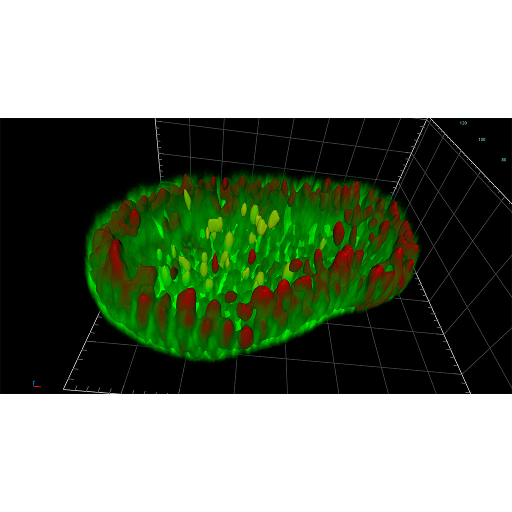
Intestinal (gut) organoids have become indispensable tools for studying both normal gut development and the mechanisms that lead to morbidities (e.g., inflammatory bowel disease). Intestinal organoids are grown from single intestinal stem cells. With the proper signaling cues applied, they eventually form organoids consisting of a single layer of enterocytes (differentiated intestinal cells) surrounding a hollow lumen that resembles the lumen of a real gut (Figure 1A).

The Wnt pathway is a well-known signaling pathway regulating intestine development and maintenance. Functions and effects of Wnt are very intricate and context-dependent (for detailed reading, see reference below). Simply put, Wnt contributes to maintaining healthy tissue stem cells and the transition and differentiation of stem cells into mature enterocytes (intestinal tissue cells). On the other hand, excessive Wnt activity (e.g., by genetic mutations) contributes to intestinal cancer.

In this application story, we showcase a simple imaging experiment performed on intestinal organoids treated with and without a Wnt-inhibiting drug, with the experimental goal to study the role of Wnt signaling in organoid formation.

  • Detailed confocal scan using Airyscan detector.
  • Figure 2A: Overview scan of organoids (widefield).

  • Figure 2B: Identification of areas of interest.

  • Figure 2C: Detailed confocal scan using Airyscan detector.

Material and Methods

For this experiment, intestinal stem cells were first equipped with fluorescent proteins Histone2B-RFP and Mem9-GFP to mark cell nuclei and membranes. Isolated single intestinal stem cells were allowed to grow to organoids for 5 days in the presence or absence of Wnt signaling pathway inhibitor IWP-2. Organoids were then fixed and antibody-stained for Aldolase B, which is a marker for differentiated enterocytes, and counterstained with DAPI (for nucleus detection).

Image acquisition was performed using a confocal ZEISS Celldiscoverer 7 that combines widefield and confocal imaging modes. Single organoids were acquired at 20X magnification with image stacks spanning the complete organoid depth.

For the acquisition of many individual organoids the ZEISS ZEN (blue edition) module "Guided Acquisition" was used. This is an automated imaging workflow consisting of three parts. A large overview scan with a low magnification (Figure 2A). An image analysis pipeline to identify areas of interest - in this case individual organoids on the overview image (Figure 2B), and a detailed scan of all identified positions (Figure 2C).​

The overview scan was performed with a 2,5x magnification in camera based widefield mode. For detailed scans (20x magnification) image stacks spanning the complete organoid depth were captured in confocal mode using the Airyscan detector.​

Figure 2D: Overview images of organoids that were treated with and without Wnt inhibitor. The images show that Wnt inhibition changes the morphology of the organoids, including size and shape. Control-treated organoids are larger and have an irregular shape.

Figure 2D: Overview images of organoids that were treated with and without Wnt inhibitor. The images show that Wnt inhibition changes the morphology of the organoids, including size and shape. Control-treated organoids are larger and have an irregular shape.

Figure 2D: Overview images of organoids that were treated with and without Wnt inhibitor. The images show that Wnt inhibition changes the morphology of the organoids, including size and shape. Control-treated organoids are larger and have an irregular shape.
Figure 2E: Control-treated organoids are larger and have an irregular shape. Figure 2E shows how Wnt inhibition presumably reduces the expression of Aldolase B.

Figure 2E: Control-treated organoids are larger and have an irregular shape. Figure 2E shows how Wnt inhibition presumably reduces the expression of Aldolase B.

Figure 2E: Control-treated organoids are larger and have an irregular shape. Figure 2E shows how Wnt inhibition presumably reduces the expression of Aldolase B.
arivis logo
arivis logo

ZEISS arivis Pro

ZEISS arivis Pro is a modular software for working with multi-channel 2D, 3D and 4D images of almost unlimited size, highly scalable and independent of local system resources. Many modern microscope systems such as high-speed confocal, light sheet / SPIM, super-resolution, electron microscopy or X-ray instruments can produce huge amounts of imaging data. ZEISS arivis Pro handles such datasets without constraints and in relatively short time.

Image Analysis Pipeline

Image Analysis Pipeline

Software Processing

First, the raw acquisition image data (one .czi file per organoid) was batch imported into a single ZEISS arivis Pro file. For both mock control and Wnt inhibitor samples, 30 organoids were included in the analysis. To reduce the data size, images were transformed to 8-bit and binned 2x2 in x-y dimensions.

​The raw image data set was then processed via image normalization in H2B-RFP, Mem9-GFP and DAPI channels to account for intensity differences between organoids and for signal intensity differences due to imaging depth.

Next, machine learning segmentation was performed to segment the outer organoid cell layer. The organoid lumen was next determined by filling inclusions in the organoid cell layer segmentation.

Nuclei were segmented with the blob finder function from H2B-RFP and DAPI channels. Nuclei within the organoid cell layer and the organoid lumen were separated into two object groups based on object distances to the organoid lumen. The cell bodies were segmented via region growing from nuclei objects within the organoid cell layer.

Finally, to facilitate better statistical analysis all object groups were stratified for single organoids. The pipeline is available for download and testing at the end of this application story.

Execution in ZEISS arivis Pro

Machine Learning

In this tutorial video, learn how to use machine learning in ZEISS arivis Pro to analyze organoids, that were imaged on the ZEISS Celldiscoverer 7 confocal microscope.

Nucleus and Cell Body Segmentation

In this tutorial video, continue with the analysis of organoids using ZEISS arivis Pro. In the previous tutorial we used machine learning to measure total volume of an organoid. Now learn how to segment the individual nuclei using the Blob Finder operation and model the cell boundaries using the Region Growing operation.

Validation

Next, we checked the validity and quality of the different segmentations applied during the analysis. The organoid cell layer and organoid lumen were segmented with the machine learning segmenter. Employing machine learning leads to superior segmentation results compared to conventional threshold-based segmentation. It allowed discrimination between cells in the cell layer (included in the objects) and lumen (excluded from the objects) based on complex image texture (Figure 3A).

Cell nuclei were segmented with blob finder segmentation. This allowed high-quality separation of nuclei despite them being densely packed in 3D and despite intensity variations. By setting up relationships between the organoid cell layer and lumen object, nuclei were then further separated into cell layer nuclei and luminal nuclei (Figure 3B). Cell bodies were segmented by region-growing from cell layer nuclei. By object filtering, they are nicely restricted to the organoid cell layer (Figure 3C).

Figure 3A: Organoid cell layer and lumen segmentation

Figure 3A: Organoid cell layer and lumen segmentation

Figure 3A: Organoid cell layer and lumen segmentation

Figure 3A:  Organoid cell layer and lumen segmentation. Cell layer overlay shown in green, lumen overlay in yellow.

Figure 3B: Nuclei in organoid cell layer and lumen

Figure 3B: Nuclei in organoid cell layer and lumen

Figure 3B: Nuclei in organoid cell layer and lumen. Cell layer nuclei shown in red, luminal nuclei shown in yellow.​

Figure 3B: Nuclei in organoid cell layer and lumen. Cell layer nuclei shown in red, luminal nuclei shown in yellow.​

Figure 3C: Cell bodies in organoid cell layer

Figure 3C: Cell bodies in organoid cell layer

Figure 3C: Cell bodies in organoid cell layer

Figure 3C: Cell bodies in organoid cell layer. Cell layer nuclei shown in red, cell layer cell bodies shown in green.

Results

Size and Roundness of Organoids

Having segmented and validated all relevant objects of interest, we now can jump into the analysis. Because of natural variation within spheroids and to allow for a simple statistical analysis, all analyses are prepared as box-whisker plots (depicting single data points, and their mean and standard deviations), comparing organoids from both experimental groups, where each dot is the data from one organoid.

First, the volumes of the full organoid (Figure 4A), the outer organoid cell layer (Figure 4B) and the organoid lumen (Figure 4C) were analyzed. There is a trend for larger volumes and particularly a larger spread of volumes in the control group, suggesting that Wnt inhibition interferes with proper growth of the spheroids. However, none of these trends were significant in a statistical t-test. Longer incubation times or including more organoids in the analysis would likely help to obtain more conclusive results.

We also observed in the initial overview image (Figure 2A) that control-treated organoids formed more amorph shapes while organoids treated with Wnt inhibitor remained spherical. ZEISS arivis Pro offers several morphological parameters to analyze such observations. Figure 4D shows a significant drop of “roundness” in control-treated samples, thus, Wnt inhibition indeed interferes with the formation of amorph organoid shapes.

Figure 4A: The volume of the full organoids.

Figure 4A: The volume of the full organoids.

Figure 4A: The volume of the full organoids.

Figure 4A: The volume of the full organoids. Single data points, mean and standard deviation are depicted. p-value from statistical t-test is shown.

Figure 4B: The volume of the organoid cell layers

Figure 4B: The volume of the organoid cell layers

Figure 4B: The volume of the organoid cell layers

Figure 4B: The volume of the organoid cell layers. Single data points, mean and standard deviation are depicted. p-value from statistical t-test is shown.

Figure 4C: The volume of the organoid inner lumen

Figure 4C: The volume of the organoid inner lumen

Figure 4C: The volume of the organoid inner lumen

Figure 4C: The volume of the organoid inner lumen. Single data points, mean and standard deviation are depicted. p-value from statistical t-test is shown.

Figure 4D: The roundness of full organoids

Figure 4D: The roundness of full organoids

Figure 4D: The roundness of full organoids

Figure 4D: The roundness of full organoids. Single data points, mean and standard are deviation depicted. p-value from statistical t-test is shown.

Cell Numbers in Different Organoid Compartments

Next, as another marker of organoid growth, we evaluated the number of cells in the different organoid compartments based on nucleus object counts. Quantification was performed for all nuclei, with cell layer nuclei and luminal nuclei processed independently. These two classes have completely different fates within the growing organoid. Luminal cells only act as a transient scaffold and eventually die off by apoptosis, while the outer layer cells form the functional epithelial tissue of the organoid.

Cell numbers are shown for the total organoid (Figure 5A), the outer organoid cell layer (Figure 5B) and the organoid lumen (Figure 5C). For all three groups, there is a significant increase in cell numbers for control-treated organoids compared to organoids exposed to Wnt inhibition (p<0.05 each in statistical t-tests). This again indicates that Wnt inhibition interferes with proper organoid outgrowth. As for organoid volumes, the spread of values (the standard deviation) is considerable. Analysis would therefore likely benefit from analyzing larger sample sizes (more spheroids in the analysis).

Figure 5A: The cell numbers of the full organoids

Figure 5A: The cell numbers of the full organoids

Figure 5A: The cell numbers of the full organoids

Figure 5A: The cell numbers of the full organoids. Single data points, mean and standard deviation are depicted. p-value from statistical t-test is shown.

Figure 5B: The cell numbers of the organoid cell layers

Figure 5B: The cell numbers of the organoid cell layers

Figure 5B: The cell numbers of the organoid cell layers

Figure 5B: The cell numbers of the organoid cell layers. Single data points, mean and standard are deviation depicted. p-value from statistical t-test is shown.

Figure 5C: The cell numbers of the organoid inner lumen

Figure 5C: The cell numbers of the organoid inner lumen

Figure 5C: The cell numbers of the organoid inner lumen

Figure 5C: The cell numbers of the organoid inner lumen. Single data points, mean and standard are deviation depicted. p-value from statistical t-test is shown.

Aldolase B Expression as a Marker for Enterocyte Differentiation​

Having described the basic morphological organoid features in the previous sections, we now turn to Aldolase B expression analysis. Aldolase B is a marker for enterocyte differentiation. During organoid maturation, intestinal stem cells should progressively transform into differentiated cells. As a result, increased Aldolase B expression is an indicator for successful organoid maturation.

Two of our object groups could theoretically be suitable for the analysis: (1) the cell layer nuclei and (2) the cell layer cell bodies. As shown in Figure 6A, Aldolase B mainly localizes to the cytosol, making the cell body objects the best suited for analysis. ZEISS arivis Pro allows extracting channel intensities from different hierarchical layers. Here, we show here the sum of Aldolase B expression for the complete organoid (Figure 6B) and the single-cell mean Aldolase B intensities measured independently on every cell (Figure 6C). In both cases, there is a strong and significant increase (p<0.001 in statistical T-tests) in organoids that were mock-treated compared to organoids treated with Wnt inhibitor. This adds further evidence that Wnt inhibition interferes with organoid maturation.

Figure 6A: Localization of Aldolase B expression in the organoids

Figure 6A: Localization of Aldolase B expression in the organoids

Figure 6A: Localization of Aldolase B expression in the organoids

Figure 6A: Localization of Aldolase B expression in the organoids. Aldolase B expression (gray) is localized to the entire cell bodies (green) rather than the nuclei (red).

Figure 6B: Total organoid Aldolase B expression

Figure 6B: Total organoid Aldolase B expression. Single data points, mean and standard deviation are depicted. p-value from statistical t-test is shown.

Figure 6C: Average cellular mean Aldolase B intensity

Figure 6C: Average cellular mean Aldolase B intensity

Figure 6C: Average cellular mean Aldolase B intensity

Figure 6C: Average cellular mean Aldolase B intensity. Single data points, mean and standard are deviation depicted. p-value from statistical t-test is shown.

Determining Aldolase B-positive Cells as an Alternative Read-out​

In the last section, we focused on measuring a continuous spectrum of Aldolase B expression; however, this has a serious drawback. It doesn’t consider that, more realistically, cells are either “positive” or “negative” for Aldolase B, as can be observed nicely in a typical organoid cross section (Figure 7A). Therefore, a more suitable analysis strategy stratifies cells into Aldolase B-positive and -negative groups, then evaluates the fraction of positive cells within an organoid.

Using this approach, a threshold must be defined that separates positive and negative populations. Figure 7B shows the bimodal distribution of Aldolase B intensity over all cells in the data set, with maxima at mean pixel intensities of 10 and 30, respectively. We selected a mean pixel intensity of 15 as a threshold for Aldolase B-positive cells. Applying this threshold generates positive and negative cells that match well with the visual impression of Aldolase B distribution in the example cross section (Figure 7A). Results are shown as total positive cells per organoid (Figure 7C) and as the percentage of positive cells per organoid (Figure 7D). Again, control-treated organoids had significantly more Aldolase B-positive cells, indicating better organoid maturation.

Figure 7A: Localization of Aldolase B expression in the organoids

Figure 7A: Localization of Aldolase B expression in the organoids

Figure 7A: Localization of Aldolase B expression in the organoids

Figure 7A: Localization of Aldolase B expression in the organoids. Aldolase B expression (grey) is localized to the entire cell bodies (green) rather than the nuclei (red).

Figure 7B: Mean Aldolase B intensity distribution of single cells

Figure 7B: Mean Aldolase B intensity distribution of single cells

Figure 7B: Mean Aldolase B intensity distribution of single cells

Figure 7B: Mean Aldolase B intensity distribution of single cells. Note the bimodal distribution curve and the threshold set between the two maxima.

Figure 7C: Number of Aldolase B-positive cells per organoid

Figure 7C: Number of Aldolase B-positive cells per organoid

Figure 7C: Number of Aldolase B-positive cells per organoid

Figure 7C: Number of Aldolase B-positive cells per organoid. Single data points, mean and standard deviation are depicted. p-value from statistical t-test is shown.

Figure 7D: Percentage of Aldolase B-positive cells per organoid

Figure 7D: Percentage of Aldolase B-positive cells per organoid

Figure 7D: Percentage of Aldolase B-positive cells per organoid

Figure 7D: Percentage of Aldolase B-positive cells per organoid. Single data points, mean and standard deviation are depicted. p-value from statistical t-test is shown.

Additional Note - Scaling Up Analysis

Once a pipeline has been created and optimized in ZEISS arivis Pro by testing on a sample set of images, it is then possible to scale up the analysis by use of the server-based VisionHub platform. As arivis VisionHub is accessed over the web, users can easily upload pipelines to their datasets, run batch analysis and then have the results readily available within the web-based user interface.​

In this study, 60 organoid samples were analyzed but it would be possible to analyze many more. arivis VisionHub watches for newly acquired images being exported from the microscope. Once the dataset is fully exported, the thumbnail becomes visible in the user interface (Figure 8A). Users can upload their pipelines and simply select datasets for analysis (Figure 8B). When the analysis is complete, the results are available as object mark-ups in the viewer (Figure 8C) and data tables are also available for download.​

Figure 8A: Datasets in VisionHub. Users can select datasets for high-throughput analysis

Figure 8A: Datasets in VisionHub. Users can select datasets for high-throughput analysis

Figure 8A: Datasets in VisionHub. Users can select datasets for high-throughput analysis

Figure 8A: Datasets in VisionHub. Users can select datasets for high-throughput analysis.

Figure 8B: Analysis scheduler. Analysis jobs are queued

Figure 8B: Analysis scheduler. Analysis jobs are queued

Figure 8B: Analysis scheduler. Analysis jobs are queued

Figure 8B: Analysis scheduler. Analysis jobs are queued.

Figure 8C: Results in VisionHub. All analysis results are available in VisionHub

Figure 8C: Results in VisionHub. All analysis results are available in VisionHub

Figure 8C: Results in VisionHub. All analysis results are available in VisionHub

Figure 8C: Results in VisionHub. All analysis results are available in VisionHub.​

Summary

In this application story we have showcased an approach to an organoid study employing a ZEISS Celldiscoverer 7 and ZEISS arivis Pro for image analysis.
Organoids place high demand on analytical techniques because of their rather complex tissue architecture (3D data sets consisting of an outer cell layer and an inner lumen) and for the multitude of differentiation markers that may be applied (organoid volume and shape, cell numbers and single-cell expression analysis of tissue). We have highlighted how all this can be accomplished with the built-in functionality of ZEISS arivis Pro.

In this experiment, we found several results that could highlight the role of Wnt signaling in intestinal organogenesis. We could validate that organoids with inhibited Wnt signaling would have decreased organoid volumes, a more immature spherical shape, fewer cell numbers and less Aldolase B expression. Aldolase B as a marker for enterocyte differentiation was reduced both in terms of total expression levels and in terms of Aldolase B-positive cell fractions.

It should be noted that only 30 organoids per sample were analyzed for the purpose of demonstrating image analysis with our software. This certainly doesn’t meet the high standards that would be required for a professional study and statistically relevant conclusions. We still believe that having this kind of “real-world” use case helps you to learn about image analysis strategies that can be applied to your own data. As always, the data set and analysis pipeline are provided here to give you the opportunity to test ZEISS arivis Pro for yourself.

How to Get Started

In this video, learn how to get started with the dataset of this case study and your trial version of ZEISS arivis Pro (both downloads are provided below). See how to load an image, load a pipeline, and how to start you analysis.

Try It for Yourself

Download all case study data and a trial version of ZEISS arivis Pro


Share this article